Web Scraping and Visualization of Rental Data in Switzerland with Python
In this article, I explain how you can:
- Get the rental data by web scraping and converting it to Pandas data frame
- Use the Geopandas library to convert maps which are in shapefile to Geopandas data frames and Geojson maps
- Make interactive Choropleth maps embedded with rental data, which looks like this (hover over the map to see average rent per room for each zip-code):
Web Scraping for rental data
If available, it is easier/recommended to use an API (similar to twitter, reddit APIs) . However, most of the websites don't have public APIs or if they have they provide very limited public access. In such cases, web scraping might be necessary.
This was the case for me when I wanted to study rental data in Switzerland. So, I decided to develop my own web crawler to get the data for analysis (not any business purposes) from Immoscout24.ch. Below I explain this web crawler. You can find the corresponding Jupyter notebook here.
First step is to download the web html pages. For instance, for city of Lausanne this is how you could do it:
import requestsfirst_page = requests.get('https://www.immoscout24.ch/en/flat/rent/city-lausanne')This snippet downloads the first page of the rental data of the city of Lausanne.
Use
html2textscript written by Aaron Swartz to convert the html page to a text file. This script gets rid of all html syntaxes:xxxxxxxxxximport html2texth = html2textc = h.html2text(first_page.text)You can
print(c)to see how it looks like. You can get meta info such as total number of pages from the first page data and then continue downloading all pages as explained in this Jupyter notebook. I have saved all pages in*.txtform.Split each txt file using regular expressions so that you can get each apartment listing: I call it
singe_apt_listingwhich is simply a string containing one single apartment listing. Here is an example of that:x### [3 rooms, 97 m²](/en/d/flat-rent-lausanne/5071748?s=2&t=1&l=2023&ct=609&ci=220&pn=10)## «Ruchonnet 24 - Appt 3 pièces au rez-de-chaussée»Av. Ruchonnet 24, 1003 Lausanne, VDClose### CHF 2,499.—BookmarkThen I use
regexin this script to extract the information such as number of rooms, area, etc. from the string above and convert it to Pandas dataframe. This step is a bit tricky as not all single apartment listings look as nice as the one above. So the script has to cover all different cases without outputing wrong data.Finally, I concatenate all single apartment data frames to a Pandas data frame which will be convenient for data analysis.
All these steps are integrated into a class
ImmoScoutwhich can be used as follows:xxxxxxxxxxfrom ImmoScout import ImmoScoutimport pandas as pd# instantiate the ImmoScout class by setting the city name and listing typelausanne = ImmoScout(city_name = 'lausanne', list_type = 'rent')# if some data is already downloaded set 'in_path' to the already saved csv file,# otherwise just set the output path, i.e., out_path to save the converted datalausanne.to_csv(in_path = '', out_path='../data/lausanne.csv')# convert the csv to pandas data framedf = pd.read_csv('../data/lausanne.csv')
Rental-Data analysis
Once you have the rental data in the form of a Pandas dataframe you can do the usual data analysis pipeline. That is, you start by preprocessing the data (handling the missing data, outliers, etc.). For the data analysis, you can include new interesting features such as rent per room, rent per area, zip code of the apartments, etc. These are all done in this notebook. Perhaps, the most tricky part of the data analysis pipeline for this example is spotting and handling the outliers (which are indeed mostly due to wrong inputs from the users). Here is the first 5 elements of the resulting dataframe:
| index | Id | SurfaceArea | NumRooms | Type | Address | Description | Rent | Bookmark | Link | RentPerArea | RentPerRoom | AreaPerRoom | ZipCode | |
|---|---|---|---|---|---|---|---|---|---|---|---|---|---|---|
| 0 | 0 | 4695812 | 41.0 | 2.0 | flat | Av. de Cour 65, 1007 Lausanne, VD | Appartement de 2 pièces au 5ème étage | NaN | New | /en/d/flat-rent-lausanne/4695812?s=2&t=1&l=202... | NaN | NaN | 20.500000 | 1007 |
| 1 | 1 | 5204125 | 21.0 | 1.5 | studio | Route Aloys-Fauquez 122, 1018 Lausanne, VD | Studio proche de toutes les commodités | 970.0 | New | /en/d/studio-rent-lausanne/5204125?s=2&t=1&l=2... | 46.190476 | 646.666667 | 14.000000 | 1018 |
| 2 | 2 | 5201717 | 95.0 | 4.0 | flat | Av. de Morges 39, 1004 Lausanne, VD | Joli appartement - centre ville proche commodités | 2085.0 | NaN | /en/d/flat-rent-lausanne/5201717?s=2&t=1&l=202... | 21.947368 | 521.250000 | 23.750000 | 1004 |
| 3 | 3 | 5201713 | 29.0 | 1.5 | flat | Ch. du Devin 57, 1012 Lausanne, VD | Quartier de Chailly, spacieux 1.5 pièce | 910.0 | NaN | /en/d/flat-rent-lausanne/5201713?s=2&t=1&l=202... | 31.379310 | 606.666667 | 19.333333 | 1012 |
| 4 | 4 | 5195729 | 11.0 | NaN | single-room | Chemin de Montolivet 19, 1006 Lausanne, VD | 1006 Lausanne - Montolivet 19 - Chambre meublé... | 560.0 | NaN | /en/d/single-room-rent-lausanne/5195729?s=2&t=... | 50.909091 | NaN | NaN | 1006 |
Let's say you are interested in rental prices distribution as a function of zip-code. Then you could use the groupBy() method of Pandas on the above dataframe as follows:
xxxxxxxxxxzipVsRentMean = df[['ZipCode', 'RentPerArea', 'RentPerRoom', 'AreaPerRoom', 'SurfaceArea']].groupby(['ZipCode'], as_index = False).mean()Here is zipVsRentMean:
| ZipCode | RentPerArea | RentPerRoom | AreaPerRoom | SurfaceArea | |
|---|---|---|---|---|---|
| 0 | 1000 | 28.458524 | 729.675634 | 25.975658 | 131.923077 |
| 1 | 1003 | 33.847367 | 956.716565 | 29.864104 | 77.057471 |
| 2 | 1004 | 29.348282 | 697.231981 | 25.349916 | 65.488971 |
| 3 | 1005 | 29.793665 | 718.242015 | 24.671657 | 73.903226 |
| 4 | 1006 | 32.542634 | 789.203604 | 26.219773 | 61.670213 |
| 5 | 1007 | 32.612209 | 774.724010 | 26.186800 | 59.460000 |
| 6 | 1010 | 28.715491 | 714.434524 | 26.260718 | 76.546512 |
| 7 | 1012 | 30.620128 | 789.353729 | 27.079760 | 69.865385 |
| 8 | 1015 | 23.448276 | 616.428571 | 24.857143 | 87.000000 |
| 9 | 1018 | 29.406521 | 668.998769 | 24.128802 | 57.859504 |
For the moment, I will drop rows of zip code 1015 as I did not have enough data points.
Read Shapefiles and convert them to Geopandas dataframes
Next, we would like to show the results of the zip code table above on a map. To this end, we first should be able to read the maps in Python. Maps are usually available in the shapefile format *.shp. Let's first download this shapefile map, and then I discuss how you could read this in Python.
Download the Switzerland's zip- code shapefiles from Swiss opendata. I have downloaded the PLZO_SHP_LV95 from here. Extract the folder, and note the address where you saved the zip-code shapefile (called PLZO_PLZ.shp) . I put it in my data folder.
Okay, now you have the shapefile. How would you read/manipulate this in Python? Luckily, the Geopandas library of Python, which is a powerful library used for geospatial data processing and analysis, has a method to convert shapefiles to geopandas dataframe:
xxxxxxxxxximport geopandas as gpdgdf = gpd.read_file('../data/PLZO_SHP_LV95/PLZO_PLZ.shp')The Coordinate Reference System (CRS) in which the data is displayed can be found by gdf.crs. I convert this to a more common CRS by the following command:
xxxxxxxxxxgdf = gdf.to_crs({'init': 'espg:4326'})Here is the first two elements of the geopandas dataframe gdf:
| UUID | OS_UUID | STATUS | INAEND | PLZ | ZUSZIFF | geometry | |
|---|---|---|---|---|---|---|---|
| 0 | {0072F991-E46D-447E-A3BE-75467DB57FFC} | {281807DC-9C0B-4364-9A55-0E8956876194} | real | nein | 3920 | 0 | POLYGON ((7.575852862870608 45.98819190048114,... |
| 1 | {C3D3316F-1DFE-468E-BFC5-5C2308743B4C} | {F065D58C-3F88-46EF-9AA0-DA0A96766333} | real | nein | 3864 | 0 | POLYGON ((8.114458487426123 46.5465644007604, ... |
The geometry column defines the shape of each polygon. Since we are only looking at the data in the city of Lausanne, I extract the data of Lausanne from gdf (note that gdf includes the data of the whole Switzerland):
xxxxxxxxxxlausanne = [1000, 1003, 1004, 1005, 1006, 1007, 1010, 1010, 1012, 1015, 1018]gdf_laus = gdf[gdf['PLZ'].isin(lausanne)]Now you can plot the zip-code map of Lausanne with the following code:
xxxxxxxxxxgdf_laus.plot()Which would result in the following figure:
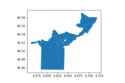
While geopandas can plot such minimal maps, I would like to have a Choropleth interactive map (where you can hover over the map see the rental results) that also looks a bit nicer than this one. To create such a map I decided to use the use the Altair library.
Create interactive Choropleth map embedded with rental data
First off, let's merge the gdf_laus dataframe which only contains geographical data with zipVsRentMean Pandas dataframe which included the rental data for each zip-code in Lausanne:
xxxxxxxxxxgdf_laus = gdf_laus.merge(zipVsRentMean, left_on='PLZ', right_on='ZipCode')This will simply add the columns of zipVsRentMean to the right of gdf_laus. Okay, now we have a geopandas dataframe gdf_laus, which includes both rental data and geographical information of Lausanne. Next, we want to visualize this on an interactive Choropleth map for which I use the Altair library.
In order for the gdf_laus data to be readable by the Altair library, we need to do some preprocessing as follows:
xxxxxxxxxximport jsonimport Altair as altjson_laus = json.loads(gdf_laus.to_json())alt_laus = alt.Data(values = json_laus['features'])alt_laus has the data form which is readable by Altair as follows:
xxxxxxxxxxalt_rentPerRoom = alt.Chart(alt_laus).mark_geoshape( stroke = 'white').encode( latitude = 'properties.y:Q', longitude = 'properties.x:Q', color = 'properties.RentPerRoom:Q').properties( width = 400, height = 500)alt_rentPerRoom # to display the mapHere is the result of the execution of this code:
We are almost there, but we need to display the zip-code on the map too. To do this, I first get the centroid of each zip-code area by the following commands:
xxxxxxxxxxgdf_laus['x'] = gdf_laus['geometry'].centroid.xgdf_laus['y'] = gdf_laus['geometry'].centroid.yNext, plot this with altair:
xxxxxxxxxxtext = alt.Chart(alt_laus).mark_text( ).encode( longitude = 'properties.x:Q', latitude = 'properties.y:Q', text = 'properties.ZipCode:Q',)Finally, combine the two maps:
xxxxxxxxxxchart = alt_rentPerRoom + textchartHere is the result. You can hover over the map to see the rent per room average in each zip-code area. We can do the same analysis for any other variable of interest (e.g., rent per surface area, etc.).
Head to this notebook for the python code that I summarized above.